4. Expedite Poisson-NMF estimation via alternating regression models

Yongjin Park

What if we apply single-effect Poisson regression alternatively? Let’s consider this parameterization of Poisson distribution: $\lambda_{ij} = \sum_{k} \beta_{ik} \theta_{jk}$ Previously, we introduced $q_{ij}^{k}$ (triplets for each gene $i$, cell $j$, and factor $k$) to derive closed-form variational update equations. But the overall complexity can increase in a cubic time. Can we factorize $q$ into two parts, like $q_{ij}^{k} = c_{ik} z_{jk}$? It will certainly lead to a more restrictive approximation objective. Perhaps, the lower-bound induced by the factored auxiliary variables will be not as tight as before. Still, we can show that some sort of alternating regression algorithm can benefit from having two factored auxiliary variables.

Let us define latent variables, $\phi_{ik} \overset{\Delta}{=} \mathbb{E}\!\left[c_{ik}\right]$ and $\rho_{jk} \overset{\Delta}{=} \mathbb{E}\!\left[z_{jk}\right]$ under variational approximation:

$$q(\mathbf{c}_{i}|\phi_{i}) = \prod_{k} \phi_{ik}^{c_{ik}}, \, q(\mathbf{z}_{j}|\rho_{j}) = \prod_{k} \rho_{jk}^{z_{jk}}$$

Regression 1: Approximation from the rows’ perspective

We want to estimate $\beta_{ik}$ given $\theta_{jk}$.

$$\sum_{i,j} Y_{ij} \ln \left( \sum_{k} \beta_{ik} \theta_{jk} \right) - \sum_{i,j,k} \beta_{ik}\theta_{jk} \ge \sum_{i,k} \sum_{j} Y_{ij} c_{ik} \ln \frac{\beta_{ik} \theta_{jk}}{c_{ik}} - \sum_{i,j,k}\beta_{ik}\theta_{jk}$$

Find the most correlated factor $k$ (softly).

$$\ln \phi_{ik} = \underbrace{\frac{\sum_{j} Y_{ij} \mathbb{E}\!\left[\ln \theta_{jk}\right]}{\sum_{j} Y_{ij}}}_{\textsf{empirical correlation}} + \underbrace{\mathbb{E}\!\left[\ln \beta_{ik}\right]}_{\textsf{memory}} + \textsf{const.}$$

with $\sum_{k} \phi_{ik} = 1$, and $$\beta_{ik} \sim \operatorname{Gamma}\left( a_{0} + \phi_{ik} \sum_{j} Y_{ij}, \, b_{0} + \sum_{j} \mathbb{E}\!\left[\theta_{jk}\right] \right)$$

$$\theta_{jk} \sim \operatorname{Gamma}\left( a_0 + \rho_{jk} \sum_{i} \phi_{ik} Y_{ij} ,\, b_0 + \sum_{i} \mathbb{E}\!\left[\beta_{ik}\right] \right)$$

Regression 2: Approximation from the columns’ perspective

$$\sum_{i,j} Y_{ij} \ln \left( \sum_{k} \beta_{ik} \theta_{jk} \right) - \sum_{i,j,k} \beta_{ik}\theta_{jk} \ge \sum_{j,k} \sum_{i} Y_{ij} z_{jk} \ln \frac{\beta_{ik} \theta_{jk}}{z_{jk}} - \sum_{i,j,k} \beta_{ik} \theta_{jk}$$

$$\ln \rho_{jk} = \underbrace{\frac{\sum_{i} Y_{ij} \mathbb{E}\!\left[\ln \beta_{ik}\right]}{\sum_{i} Y_{ij}}}_{\textsf{empirical correlation}} + \underbrace{\mathbb{E}\!\left[\ln \theta_{jk}\right]}_{\textsf{memory}} + \textsf{const.}$$

where $\sum_{k} \rho_{jk} = 1$, and

$$\theta_{jk} \sim \operatorname{Gamma}\left( a_{0} + \rho_{jk} \sum_{i} Y_{ij},\, b_{0} + \sum_{i} \mathbb{E}\!\left[\beta_{ik}\right] \right)$$

$$\beta_{ik} \sim \operatorname{Gamma}\left( a_{0} + \phi_{ik} \sum_{j} Y_{ij} \rho_{jk}, \, b_{0} + \sum_{j} \mathbb{E}\!\left[\theta_{jk}\right] \right)$$

Final remark

As a result, we will maximize the following lower-bound:

$$L \ge \sum_{i,j,k} Y_{ij} \phi_{ik} \rho_{jk} \ln \frac{\beta_{ik} \theta_{jk}}{\phi_{ik} \rho_{jk}} - \sum_{i,j,k} \beta_{ik} \theta_{jk}.$$

Example

library(asapR)
library(pheatmap)

set.seed(1331)
d <- 500
n <- 5000
.rnorm <- function(d1,d2) matrix(rnorm(d1 * d2), d1, d2)

uu <- pmax(.rnorm(d, 5), 0)
vv <- pmax(.rnorm(n, 5), 0)
Y <- uu %*% t(vv) + pmax(.rnorm(d, n), 0)

system.time(out <- asap_fit_pmf(Y, maxK=7))

##    user  system elapsed 
## 206.659 327.108  41.356

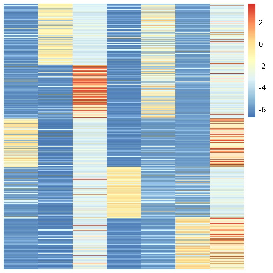
u.order <- order(apply(uu, 1, which.max))
pheatmap(out$log.beta[u.order, ], Rowv=NA, Colv=NA, cluster_rows = F, cluster_cols = F)

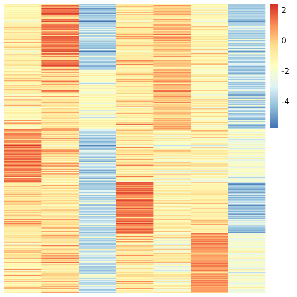
v.order <- order(apply(vv, 1, which.max))
pheatmap(out$log.theta[v.order, ], Rowv=NA, Colv=NA, cluster_rows = F, cluster_cols = F)