2. Batch correction within each pseudobulk sample

A generative scheme for a single-cell count matrix with multiplicative batch effects

We encounter single-cell expression data consisting of multiple batches. One of the primary goals is to identify cell types (clusters/factors) and cell-type-specific gene expression patterns. However, distinguishing batch-specific and cell-type-specific genes only by a factorization method is challenging and often not identifiable from data alone. For each gene $g$ and cell $j$ , the gene expression $Y_{gj}$ were sampled from Poisson distribution with the rate parameter:

$\lambda_{gj} = \lambda_{gj}^{\textsf{unbiased}} \times \prod_{k} \delta_{gk}^{X_{kj}},$

affected by the batch effects $\delta_{gk}$ . More formally, letting $X_{kj}$ be a batch membership matrix, assigning a cell $j$ to a batch $k$ if and only if $X_{kj}=1$ , we assume the average gene expression rates are linearly affected by in the log-transformed space:

$\mathbb{E}\!\left[\ln Y_{gj}\right] = \ln \left( \sum_{t} \beta_{gt} \theta_{jt} \right) + \sum_{k} \ln\delta_{gk} X_{kj}.$

library(pheatmap)
set.seed(1331)

m <- 500 # genes
n <- 1000 # cells
nb <- 2 # batches

## 1. batch membership
X <- matrix(0, n, nb)
batch <- sample(nb, n, replace = TRUE)
for(b in 1:nb){
    X[batch == b, b] <- 1
}

## 2. batch effects
W.true <- matrix(rnorm(m*nb), m, nb)
ln.delta <- apply(W.true %*% t(X), 2, scale)

## 3. true effects
K <- 5
.beta <- matrix(rgamma(m * K, 1), m, K)
.theta <- matrix(rgamma(n * K, 1), n, K)
lambda.true <- .beta %*% t(.theta)
kk <- apply(.theta, 1, which.max)

lambda <- lambda.true * exp(ln.delta)
yy <- apply(lambda, 2, function(l) sapply(l, rpois, n=1))
oo <- order(apply(t(.theta), 2, which.max))

If we can accurately estimate a true batch effect matrix, say $\delta_{gk}$ , it is straightforward to adjust the difference between batches. How can we identify the true batch effect $\delta_{gk}$ for all the genes $g$ specifically expressed in the batch $k$ ? If we match cells $i$ and $j$ sampled from the batches $a$ and $b$ , respectively, we expect the batch-specific difference $\delta_{ga} \neq \delta_{gk}$ will persist and even amplify, but the difference originated from cell types will vanish. This problem is equivalent to estimating the potential outcome of gene expressions in each batch $k$ , $\mathbb{E}\!\left[Y_{gj}^{(k)}\right]$ .

A causal inference approach to identify batch effects

To dissect batch-specific effect in a causal inference (potential outcome) framework, we assume our confounding variables $Q$ are well-distributed across different batches:

Overlap: $0 < p(X_{kj}=1|Q) < 1$ for all $k$ .

Moreover, we assume these covariates are sufficient enough to induce conditional dependence between potential (imputed) gene expression and batch assignment mechanisms:

Strong ignorability: $(Y(k), Y(k')) \perp\!\!\!\perp X | Q$ for all $k,k'$ pairs.

Estimation of the batch effects by matching

Suppose we can counterfactually estimate gene expressions of a certain cell $j$ if the cell was measured in different batches other than the observed batch $k$ .

$Z_{gj} = \frac{ \sum_{i} (1 - X_{ik}) w_{ji} Y_{gi} }{ \sum_{i} (1 - X_{ik}) w_{ji} }$

Like many other batch correction methods invented for single-cell RNA-seq analysis, we will assume $Z_{gj}$ reliably contain biologically-relevant cell state information while excluding the batch-specific effects to which the cell $j$ belong.

Observed log-likelihood: $\prod_{j} p(Y_{gj}|\mu_{gs},\delta_{gk},X_{jk}) =\prod_{j} \operatorname{Poisson}(Y_{gj}|\mu_{gs} \sum_{k} \delta_{gk} X_{jk})$

Counterfactual log-likelihood: $\prod_{j} p(Z_{gj}|\mu_{gs}, \gamma_{gs}) = \prod_{j} \operatorname{Poisson}(Z_{gj}|\mu_{gs} \gamma_{gs})$

Local update: Maximize batch $s$ -specific parameters

$\mathbb{E}\!\left[\mu_{gs}\right] \approx \frac{ \sum_{j \in \mathcal{C}_{s}} Y_{gj} + \sum_{j \in \mathcal{C}_{s}} Z_{gj} } {\sum_{k} \delta_{gk} n_{sk} + n_{s} \gamma_{gs}}$

Letting $p_{sk} = n_{sk} / n_{s}$ , $\mu_{gs} \gets \frac{ \bar{Y}_{gs} + \bar{Z}_{gs}} {\sum_{k} \delta_{gk} p_{sk} + \gamma_{gs}}$

If $\delta_{gk} \to 0$ and $p_{sk}=1$ , meaning that this sample $s$ is just sampled from the batch $k$ only, $\mu_{gs} \to \bar{Y}_{gs} + \bar{Z}_{gs}$ and $\bar{Y}_{gs} \to \bar{Y}_{gsk} = 0$ . Therefore, $\mu_{gs} \to \bar{Z}_{gs}$ .

Global update

$\mathbb{E}\!\left[\delta_{gk}\right] \approx \frac{\sum_{s} \sum_{j \in \mathcal{C}_{s}} X_{kj} Y_{gj}}{\sum_{s} \mu_{gs} \sum_{j \in \mathcal{C}_{s}} X_{kj}}$

$\delta_{gk} \gets \frac{\sum_{s} \bar{Y}_{gsk} n_{sk}} {\sum_{s} \mu_{gs} n_{sk}}$

If $\bar{Y}_{gsk} \to \mu_{gs}$ for all $s$ , $\delta_{gk} \to 1$ . If $\bar{Y}_{gsk} < \mu_{gs}$ in all $s$ , $\delta_{gk} < 1$ . If $\bar{Y}_{gsk} \to 0$ for all $s$ , $\delta_{gk} \to 0$ .

Algorithm

Initialize batch effect $\delta_{gk} \gets 1$ for each gene $g$ and batch $k$
Initialize $\gamma_{gs} \gets 1$ for each sample $s$
Static global stat: $S_{gk} \gets 0$
For each pseudo-bulk sample $s$ with cells $\mathcal{C}_{s}$ ,
- $n_{sk} \gets \sum_{j \in \mathcal{C}_{s}} X_{kj}$ , $n_{s} \gets \sum_{k} n_{sk}$ , $p_{sk} \gets n_{sk}/n_{s}$
- $\bar{Y}_{gs} \gets \sum_{j \in \mathcal{C}_{s}} Y_{gj} / n_{s}$
- $\bar{Y}_{gsk} \gets \sum_{j \in \mathcal{C}_{s}} Y_{gj} X_{kj} / n_{s}$
- $\bar{Z}_{gs} \gets \sum_{j \in \mathcal{C}_{s}} Z_{gj} / n_{s}$ after matching and imputation
- $S_{gk} \gets S_{gk} + \bar{Y}_{gsk} n_{sk}$
Iterative-updated global stat: $T_{gk} \gets 0$
(Local step) For each PB sample $s$ :
- $\bar{\delta}_{gs} \gets \sum_{k} \delta_{gk} p_{sk}$
- $\mu_{gs} \gets (\bar{Y}_{gs} + \bar{Z}_{gs}) / (\gamma_{gs} + \bar{\delta}_{gs})$
- $\gamma_{gs} \gets (\bar{Y}_{gs})/(\mu_{gs})$
- For each $k$ : $T_{gk} \gets T_{gk} + \mu_{gs} n_{sk}$
(Global step) For each batch $k$ :
- $\delta_{gk} \gets S_{gk} / T_{gk}$
Repeat the previous three steps (5-7) until convergence

A toy example

## 1. project
K <- 5
R <- matrix(rnorm(m * K), K, m)
Q.raw <- R %*% yy # K x n

Before we adjust batch membership in the random projection matrix:

cor(t(Q.raw), X)

       [,1]       [,2]

[1,] 0.7617260 -0.7617260 [2,] 0.8283630 -0.8283630 [3,] 0.8099248 -0.8099248 [4,] -0.7250199 0.7250199 [5,] 0.6651915 -0.6651915

## 2. regress out
##
##  X theta = X inv(X'X) X' Y
##          = U D V' V inv(D^2) V' (U D V')' Y
##          = U inv(D) V' V D U' Y
##          = U U' Y

x.svd <- svd(X)
U <- x.svd$u
U.t <- t(x.svd$u)

Q.t <- t(Q.raw)
Q.t <- Q.t - U %*% U.t %*% Q.t
Q <- t(Q.t)

After we adjust the batch effects:

cor(Q.t, X)

          [,1]          [,2]

[1,] -2.276319e-16 2.276319e-16 [2,] -5.524025e-16 5.524025e-16 [3,] -2.934286e-16 2.934286e-16 [4,] 3.075415e-16 -3.075415e-16 [5,] -3.636223e-16 3.636223e-16

q.svd <- svd(Q)

## 3. sorting
B <- (sign(q.svd$v) + 1)/2
ss <- apply(sweep(B, 2, 2^(seq(0,K-1)), `*`), 1, sum) + 1

feat.dn <- apply(Q, 2, function(x) x / sqrt(sum(x^2)))
knn <- 3
d <- nrow(feat.dn)

library(RcppAnnoy)
## a. construct dictionary for each batch
dict.list <- lapply(sort(unique(batch)),
                    function(b) { new(AnnoyAngular, d) })

for(j in 1:length(batch)){
    b <- batch[j]
    dict.list[[b]]$addItem(j, feat.dn[,j])
}

for(dd in dict.list){
    dd$build(50)
}

## b. a simplified routine to retrieve and estimate counterfactual y
.counterfactual <- function(j){
    v <- feat.dn[,j]

    nn <- c()
    dd <- c()

    for(k in 1:nb){
        if(k == batch[j]) next
        .nn <- dict.list[[k]]$getNNsByVector(v, knn)
        .dd <- apply(feat.dn[, .nn], 2, function(u) sum((u - v)^2))
        nn <- c(nn, .nn)
        dd <- c(dd, .dd)
    }

    w <- exp(-(dd - max(dd)))
    w <- w/sum(w)

    yy[, nn, drop = FALSE] %*% matrix(w, ncol=1)
}

ngene <- nrow(yy)
nbatch <- ncol(X)
nsample <- max(ss)

.delta.db <- matrix(1, ngene, nbatch)       # gene x batch effects
.delta.num.db <- matrix(0, ngene, nbatch)    # gene x batch numerators
.delta.denom.db <- matrix(0, ngene, nbatch)  # gene x batch denominators

.prob.bs <- matrix(0, nbatch, nsample)      # batch x sample probabilities
.size.bs <- matrix(0, nbatch, nsample)      # batch x sample freq
.ybar.ds <- matrix(0, ngene, nsample)       # gene x sample observed average
.zbar.ds <- matrix(0, ngene, nsample)       # gene x sample imputed average
.mu.ds <- matrix(1, ngene, nsample)         # gene x sample adjusted average

## Precalculate some statistics
for(s in 1:nsample){
    if(sum(ss == s) < 1) next

    .yy <- yy[, ss == s, drop = FALSE]
    .zz <- do.call(cbind, lapply(which(ss == s), .counterfactual))

    .ybar.ds[,s] <- apply(.yy, 1, mean)
    .zbar.ds[,s] <- apply(.zz, 1, mean)
    .prob.bs[,s] <- colMeans(X[ss == s, ])
    .size.bs[,s] <- colSums(X[ss == s, ])

    .y.dsb <- yy[, ss == s, drop = FALSE] %*% X[ss == s, , drop = FALSE]
    .delta.num.db <- .delta.num.db + .y.dsb
}

.gamma.ds <- matrix(1, ngene, nsample)

for(iter in 1:100){
    .mu.ds <- (.ybar.ds + .zbar.ds) / (.delta.db %*% .prob.bs + .gamma.ds + 1e-8)
    .gamma.ds <- .zbar.ds / (.mu.ds + 1e-8)
    .delta.db <- .delta.num.db / (.mu.ds %*% t(.size.bs) + 1e-8)
}

Can we recover the original batch effects?

par(mfrow=c(1,2))
plot(.delta.db[,1], W.true[,1], pch=19, xlab="estimated delta", ylab="true delta effect", main="batch1")
plot(.delta.db[,2], W.true[,2], pch=19, xlab="estimated delta", ylab="true delta effect", main="batch2")

Are they independent of the cell type effects?

y.true <- sweep(lambda.true %*% X, 2, colSums(X), `/`)
par(mfrow=c(1,2))
plot(.delta.db[,1], y.true[,1], pch=19, xlab="estimated delta", ylab="true y mean", main="batch1")
plot(.delta.db[,2], y.true[,2], pch=19, xlab="estimated delta", ylab="true y mean", main="batch2")

While adjusting the estimated batch effects, can we recover the unbiased cell type effects? The following is before adjustment:

ybar <- sweep(yy %*% X, 2, colSums(X), `/`)
par(mfrow=c(1,2))
plot(ybar[,1], y.true[,1], pch=19, xlab="sample mean", ylab="true y mean", log="x", main="batch1")
plot(ybar[,2], y.true[,2], pch=19, xlab="sample mean", ylab="true y mean", log="x", main="batch2")

Here, we adjusted the batch effects:

ybar.adj <- sweep((yy / .delta.db[, batch]) %*% X, 2, colSums(X), `/`)
par(mfrow=c(1,2))
plot(ybar.adj[,1], y.true[,1], pch=19, xlab="adjusted sample mean", ylab="true y mean", log="x", main="batch1")
plot(ybar.adj[,2], y.true[,2], pch=19, xlab="adjusted sample mean", ylab="true y mean", log="x", main="batch2")

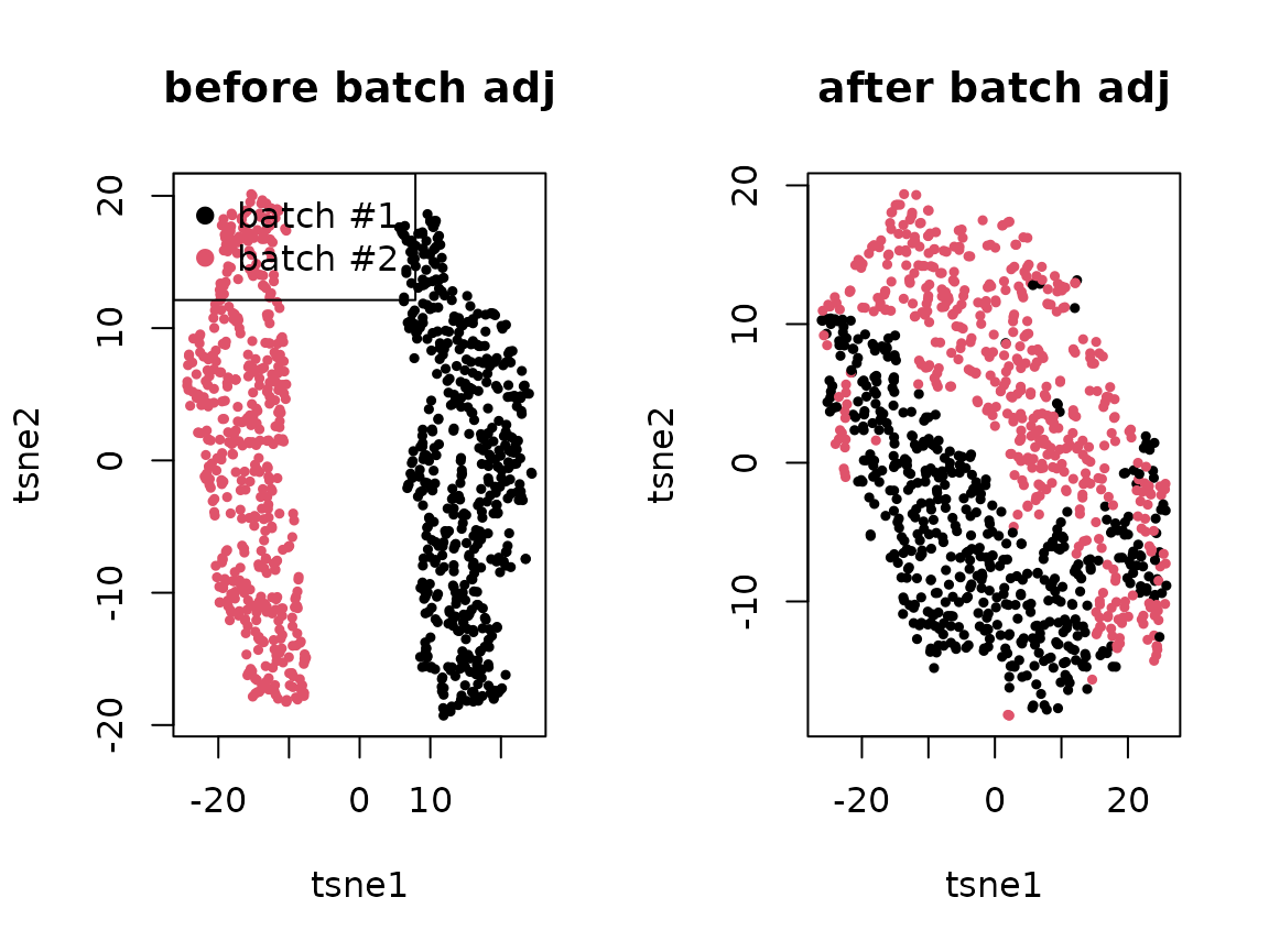
par(mfrow=c(1,2))
.tsne <- Rtsne::Rtsne(log(1 + t(yy)), num_threads=4)$Y
plot(.tsne[,1], .tsne[,2], col=batch, pch=19, cex=.5, main="before batch adj",
     xlab = "tsne1", ylab = "tsne2")
legend("topleft", c("batch #1", "batch #2"), col=1:2, pch=19)
.tsne <- Rtsne::Rtsne(log(1 + t(yy/.delta.db[,batch])), num_threads=4)$Y
plot(.tsne[,1], .tsne[,2], col=batch, pch=19, cex=.5, main="after batch adj",
     xlab = "tsne1", ylab = "tsne2")

Yongjin Park